Replicating Airbnb's Amenity Detection with Detectron2

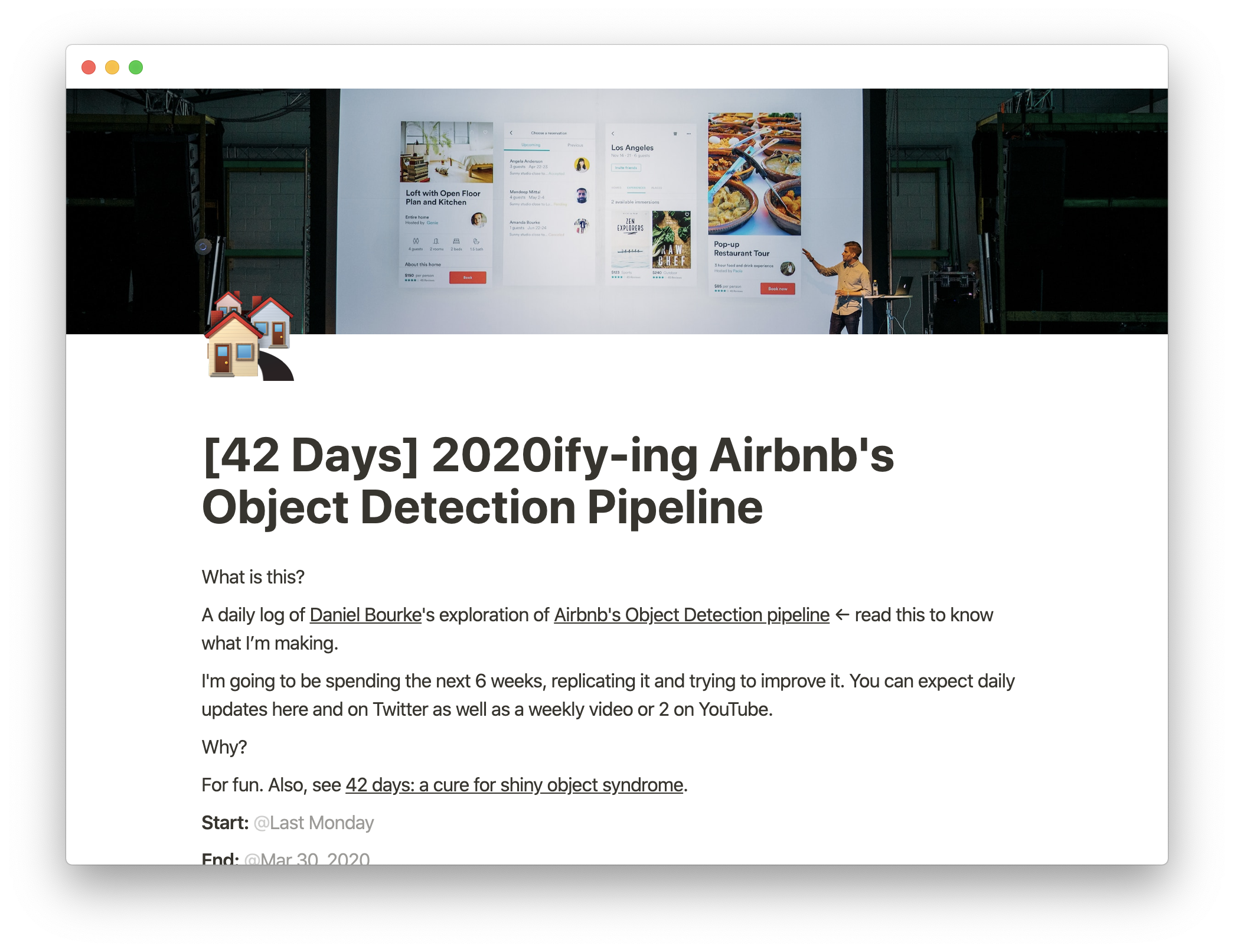
A couple of months ago, I read an article by Airbnb’s engineering team which described how they used computer vision to detect amenities in photos.

The article read like a recipe. A machine learning recipe.

Like any budding chef (or machine learner), I decided to reproduce it and add a few of my own flavours.

Wait.

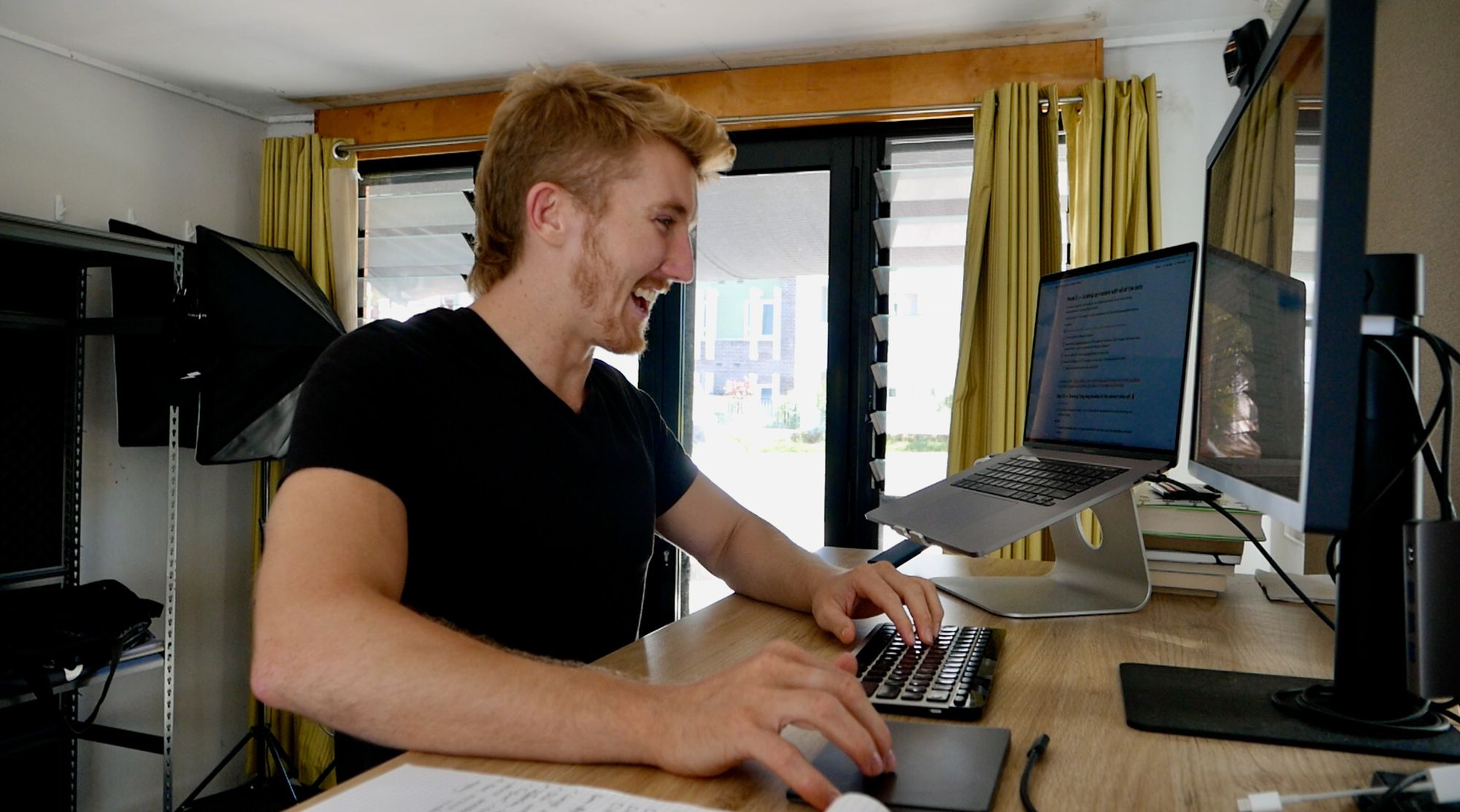
What’s an amenity?

Think of something useful in a room. Say an oven in a kitchen or a shower in a bathroom.

Why would detecting these in images be helpful?

This is where the business use-case comes in. You’ll often see tutorial computer vision models being built on datasets like MNIST (photos of hand-written digits) but it’s hard to translate those kinds of problems to a business use-case (unless you’re a postal service in the business of detecting handwritten digits).

If you’ve seen Airbnb’s website, there are lots of photos of homes and places to stay. Alongside these places to stay are text-based details describing the finer-details. Like whether or not the listing you’re looking at has a jacuzzi or not.

How about an example?

Let’s say you want to list your home on Airbnb. You might upload some photos and fill out a few details about it. But chances are, since you know your own place so well, you might miss a few things.

This is where automatic amenity detection could be helpful.

As you upload images to Airbnb, a computer vision machine learning model looks at the images, tries to find the key amenities in each one and adds them to your listing automatically.

Of course, it could verify with you that its predictions were correct before they actually go live. But having it happen automatically would help to make sure the information on each listing is as filled out as possible.

Having as detailed information as possible about each listing means the people searching for places with specific criteria. So the young couple after a nice weekend splitting their time between the jacuzzi and in front of the fireplace can find what they’re looking for.

A note to the reader, treat this article as a high-level narrative of what happened mixed with a splash of tech. For the nerds like me, the code is available in the example Google Colab Notebook.

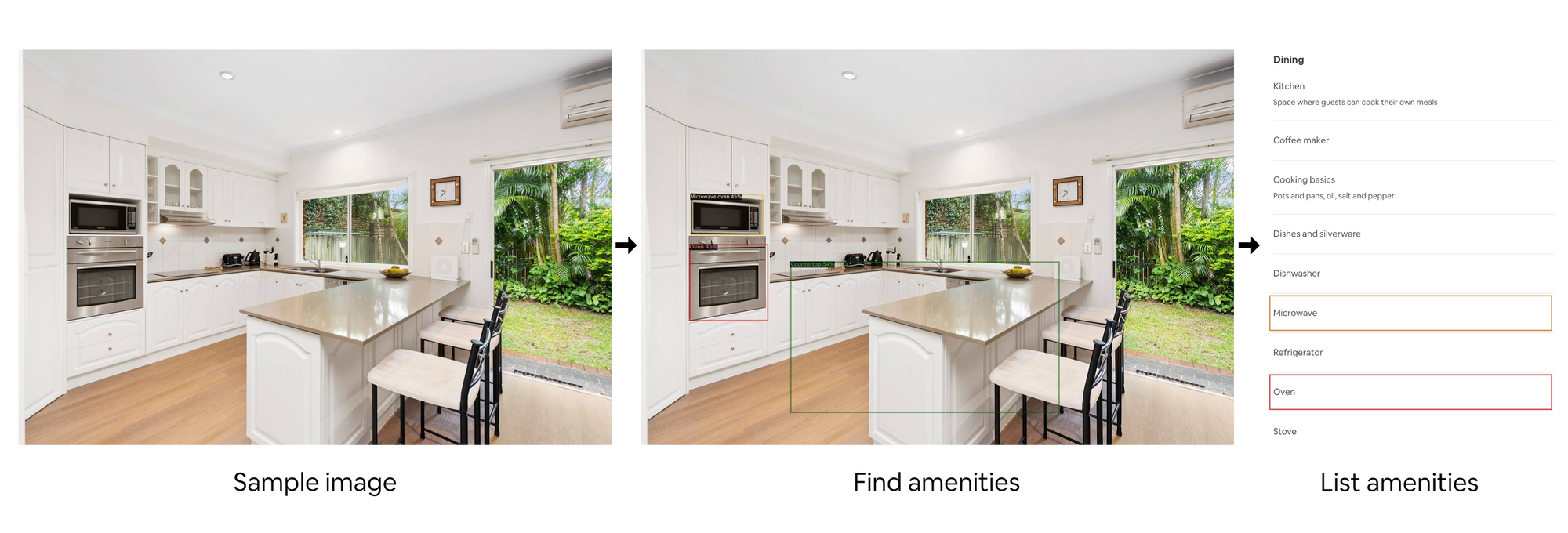
The 42-day project: learning by doing

Before starting this project I was like a chef with a set of untouched knives. Or in my case, a machine learning engineer who hadn’t used Detectron2, Weights & Biases, Streamlit or very much of PyTorch yet (these are all machine learning tools).

I’ve found I learn best about things when building things. You might be the same.

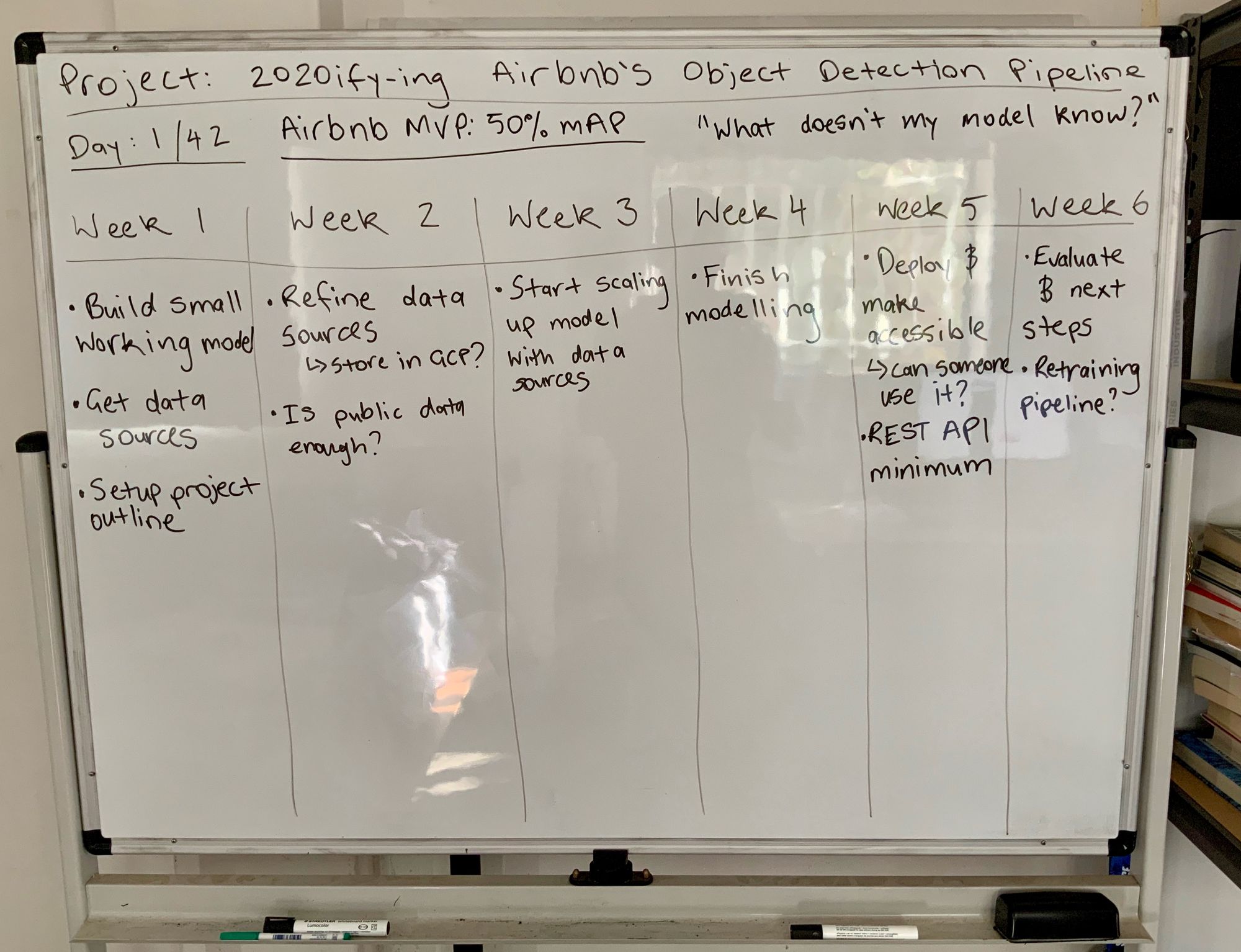
So I cracked open a Notion document, wrote down some criteria, and put together a little 6-week outline on my whiteboard.

Why 6-weeks?

Because 42-days feels like enough time to get something significant done but not so long that it takes over your life.

Anyway.

I figured I’d spend 6-weeks or so (3ish hours per day) replicating Airbnb’s amenity detection with the set of tools I’d been wanting to try.

Worst case, I learn a few things and if all fails, it’s only 6-weeks.

Best case, I learn a few things and got a pretty cool machine learning app built.

Either way, there’d be a story to tell (you’re reading it).

Breaking it down

This fun little graphic breaks the major steps taken in the experiment.

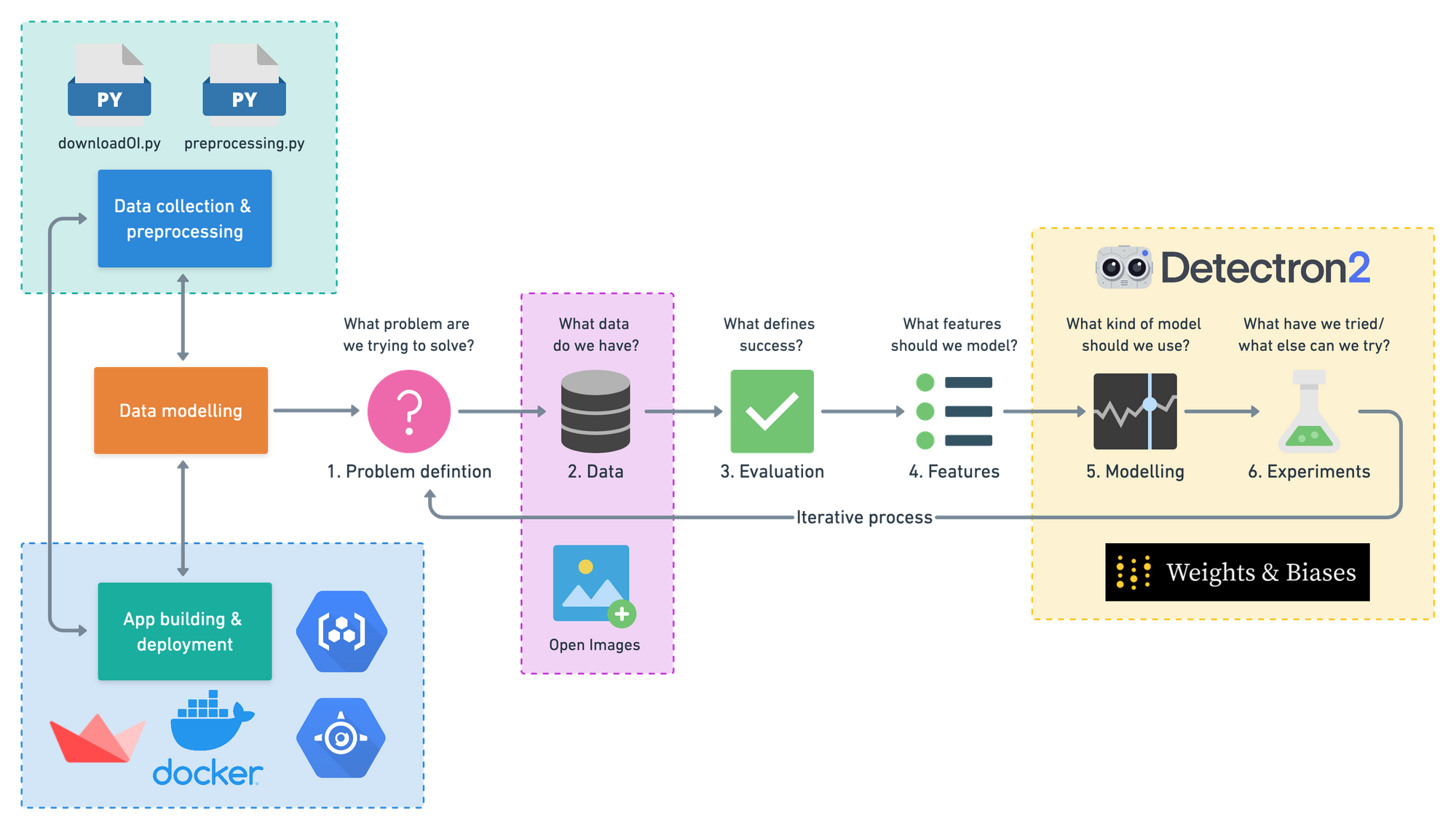
Sometimes text is easier to read than images full of other images.

Replicating Airbnb’s amenity detection with Detectron2 recipe:

1. Collect data with downloadOI.py (a script for downloading certain images from the Open Images).
2. Preprocess data with preprocessing.py (a custom script with functions for turning Open Images images and labels into Detectron2 style data inputs).
3. Model data with Detectron2.
4. Track modelling experiments with Weights & Biases.
5. Create a user-facing app with Streamlit.
6. Deploy app and model with Docker, GCR (Google Container Registry) and Google App Engine.

We’ll use these to drive the rest of the article. Let’s get into it.

Data Collection: Downloading Airbnb target images and labels files from Open Images

• Ingredients: 1 x download script, 4 x label files, 38,000+ x Open Images
• Time: 1 week
• Cost: $0
• Utensils: Google Colab, local machine

Like all machine learning projects, it begins and ends with the data.

The Airbnb article mentioned to build their proof of concept, they used 32k public images and 43k internal images.

Alas, the first roadblock.

Of course, other than a phone call interview for a technical support role in 2016, I have no affiliation with Airbnb internally, so the internal images were off the table.

The good news was the 32k public images they used were from Open Images (a massive free and open-source resource of millions of images from 600+ categories of different things).

However, if you look at Open Images, you’ll find there are over a 1-million different images.

So what’s the deal?

Why did Airbnb only use 32k?

Good question.

It’s because they were only interested in images relevant to their business use-case (images of rooms containing common amenities).

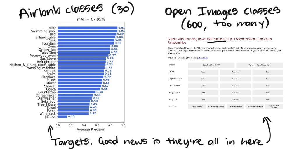
Knowing the target classes Airbnb were most concerned about, I thought, surely there was a way to only download the images from Open Images you care about (and not the entire 1.9 million+, 500GB+ dataset).

Turns out there was.

After a bit of searching, I found a great guide from LearnOpenCV on how to download only images from a list of target classes.

Specifically, a script called downloadOI.py which allowed you to define what classes you were after and from which dataset.

Let’s see an example.

!python3 downloadOI.py --dataset "validation" --classes "Kitchen & dining room table"

This line says, “get the images with kitchen & dining room tables in them from the validation set of Open Images.”

Running the line of code above will download all of the images from the target class(es) into a folder with the same name as the target dataset.

# What your image folder(s) look like after using downloadOI.py
validation <- top file 
│   kitchen_&_dining_room_table_image_1.jpg <- image 1
│   kitchen_&_dining_room_table_image_2.jpg <- image 2
|   ... <- more images...

The original downloadOI.py from LearnOpenCV script worked great, it even generated labels as the images downloaded. But after a little experimentation, I found these labels incompatible for working with Detectron2.

So I scrapped the label creation on download and modified the script to only download images. I decided I’d write my own label creating code.

Being able to download images: check.

Now for the labels.

The Open Images labels are a bit more accessible and can be downloaded by clicking the specific download links on the Open Images download page or by running the following code (tidbit: scroll to the bottom of the download page to see information about the labels).

# Open Images training dataset bounding boxes (1.11G)
!wget https://storage.googleapis.com/openimages/2018_04/train/train-annotations-bbox.csv

# Open Images validation dataset bounding boxes (23.94M)
!wget https://storage.googleapis.com/openimages/v5/validation-annotations-bbox.csv
    
# Open Images testing bounding boxes (73.89M)
!wget https://storage.googleapis.com/openimages/v5/test-annotations-bbox.csv

# Class names of images (11.73K)
!wget https://storage.googleapis.com/openimages/v5/class-descriptions-boxable.csv

The first stage of data collection resulted in acquiring the following files.

• 1 class (coffeemaker) of images from Open Images train, validation and test sets.
• Training (train-annotations-bbox.csv), validation (validation-annotations-bbox.csv) and test (test-annotations-bbox.csv) set bounding box image labels.
• The descriptions of different Open Images classes (class-descriptions-boxable.csv)

Why only 1 class?

My plan was to start small. Get data preprocessing and a Detectron2 model working with 1 class and then scale up when needed.

Data Preparation: Getting Open Images data and labels into Detectron2 style inputs

• Ingredients: 5 x preprocessing functions, 4 x label files, 38,000+ x Open Images, Detectron2 documentation
• Time: 1 week +/- 1 week
• Cost: $0
• Utensils: Google Colab, local machine

The trick here was remixing the data files I had (a handful of label CSVs and a couple of folders of images) into Detectron2 style labels.

I found out if you want to use your own custom data with Detectron2, you’ll need to turn it into a list of dictionaries. Where each dictionary is the information associated with 1 image.

Let’s see an example.

Now, what do each of these fields mean?

• annotations (list): all of the annotations (labels) on an image, a single image may have more than one of these. For object detection (our use case), it contains:
• bbox (list of int): the coordinates in pixel values of a bounding box.
• bbox_mode (Enum): the order and scale of the pixel values in bbox, see more in the docs.
• category_id (int): the numerical mapping of the category of the object inside bbox, example {'coffeemaker':0, 'fireplace':1}.
• file_name (str): string filepath to target image.
• height (int): height of target image.
• width (int): width of target image.
• image_id (int): unique image identifier, used during evaluation to identify images.

If you want to build your own object detection model with Detectron2, you’ll need one of these for each of your images.

As we’ll see later, one of my first major goals for the project was getting a small model (always start small) running on custom data.

Starting small meant writing data preparation functions for 1 class of images (coffeemaker) and making sure they worked with Detectron2.

Getting the image IDs

The good thing about downloading data from Open Images is every image has a unique identifier.

For example, 1e646e27c250cd56.jpg is a picture of a coffeemaker and its unique identifier, 1e646e27c250cd56, is different from every other image in Open Images.

So I wrote a function called get_image_ids() which would go through a folder and return a list of all the unique image IDs in that folder.

This meant I knew all of the images I was dealing with.

Formatting the existing annotations files

Why is having a list of the unique image IDs helpful?

Here’s why.

When you download the label files from Open Images and import them using pandas, they look like this.

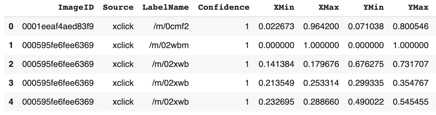
See the ImageID column? That’s where we can match up the list of image IDs we’ve downloaded from Open Images.

But wait.

Why do this?

Two reasons.

The first being, we need the extra information such as the XMin, XMax, YMin and YMax coordinates (we’ll see an example of this soon).

The second being, downloading the annotations files from Open Images results in us getting the annotations for every single image in the database but we’re only interested in the annotations for our target images.

You may have noticed the LabelName column has some weird values like /m/0cmf2 and /m/02xwb, well it turns out, these are codes too.

Here’s where the mysterious class-descriptions-boxable.csv comes into play.

Let’s have a look at it.

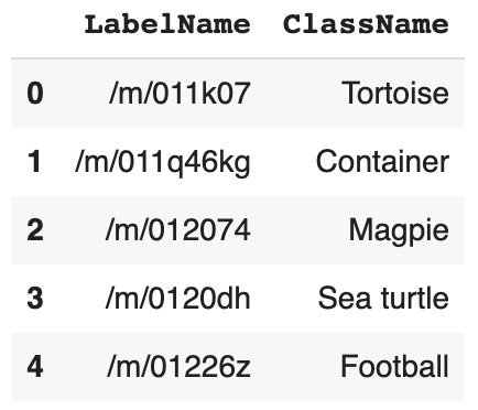
I don’t know about you but the ClassName’s look much better than /m/0cmf2 and /m/02xwb.

Having these along with a list of target classes, in my case, only coffeemaker, to begin with, I had all the ingredients needed to create format_annotations().

In a long-winded sentence, format_annotations() takes an existing annotations file downloaded from Open Images, such as, validation-annotations-bbox.csvadds some useful information to it (such as human-readable class names and a numerical categorical ID for each class) and removes unneeded rows (images we're not focused on).

Let’s see a little highlight.

Running this function takes care of the category_id portion of our label dictionaries. And as for removing all non-coffeemaker rows,validation-annotations-bbox.csv gets reduced from 303,980 rows to 62 rows.

We’re making progress but we’re not finished yet.

Converting the bounding box pixel values from relative to absolute

You might be wondering about what bbox_mode in the label dictionary means.

If not, I'll show you how I took care of it anyway.

bbox and bbox_mode are dance partners.

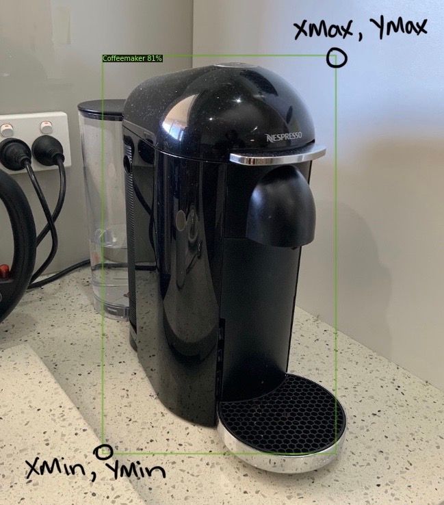
Take another look at the Open Images labels and you’ll see the columns XMin, XMax, YMin and YMax. These are the relative pixel coordinates of each bounding box on the image.

Relative pixel coordinates means to find the actual pixel values of where each corner of the target bounding box appears you have to multiply the XMin, XMax values by the width of the image and the YMin and YMax values by the height of the image.

Knowing this is important because Detectron2 currently only supports absolute pixel values (the result of multiplying a relative pixel value by the height or width).

The order matters too.

Open Images bounding box come in the order XMin, XMax, YMin, YMax but Detectron2 requires XMin, YMin, XMax, YMax.

This is where the function rel_to_absolute() comes in.

It uses an image’s height, width and existing bounding box coordinates and uses them to convert the Open Images style coordinates to Detectron2 style coordinates.

Once we’ve done the conversion, thebboxparameter is taken care of in the form ofbbox_mode (BoxMode.XYXY_ABS).

Creating image dictionaries (Detectron2-style labels)

So far we’ve made a few helper functions. Time to put it all together. The good news is, we’ve done most of the grunt work.

The penultimate (second to last, yes, there’s one more) helper function is get_image_dicts().

It takes a target image folder, a related annotation file and a list of target classes and then uses the functions above, get_image_ids(), format_annotations() and rel_to_absolute() plus a little logic of own to create Detectron2 style labels (a list of dictionaries).

Woah. That was a mouthful.

At this point, the reader is reminded if you want to see this in action, check the example Google Colab notebook.

For now, we’ll continue the story.

Oh yeah, there’s one more thing you should know about get_image_dicts(), once it creates the list of image dictionaries, it saves them to a JSON file. This makes sure we can use them later.

# Create list of validation image dictionaries
val_img_dicts = get_image_dicts(image_folder="validation", 
                                annotation_file="val-annotations.csv", 
                                target_classes=target_classes)

>>> Using validation-annotations-bbox.csv for annotations...
On dataset: validation/
Classes we're using:
Coffeemaker    21
Name: ClassName, dtype: int64
Total number of images: 21
Saving labels to: validation/valid_labels.json... 
Showing an example:
[{'annotations': [{'bbox': [2.0, 173.0, 1008.0, 768.0],
                   'bbox_mode': <BoxMode.XYXY_ABS: 0>,
                   'category_id': 1}],
  'file_name': './cmaker-fireplace-valid/c86feb2143de77e7.jpg',
  'height': 768,
  'image_id': 50,
  'width': 1024}]
CPU times: user 1.46 s, sys: 25.1 ms, total: 1.49 s
Wall time: 1.49 

And by later, I mean when you register a dataset with Detectron2.

For some reason, when you register a dataset with Detectron2, and the dataset requires some preprocessing, the preprocessing must be done with a lambda function and thus can only take one parameter.

Enter load_json_labels(), the final helper function which imports a JSON file (remember how we saved them for later) from a target image folder.

The trick you’ll want to pay attention to here is making sure if you do save your image dictionaries to file and reimport them, you ensure the bbox_mode is formatted as a Detectron2 style BoxMode.

BoxMode is a Python enum type, a special type which in my experience doesn't save itself to JSON very well (you might be able to enlighten me here).

Boom.

Data preprocessing done. All we’ve got to do is register our datasets with Detectron2 and we’re ready to start modeling.

Wait, why do we need to register a dataset with Detectron2?

Now, I’m not entirely sure of this. But once you do, the registered dataset becomes semi-immutable (can’t be easily changed).

This seems like a great idea to prevent dataset mismatches in the future.

A little call of DatasetCatalog.register()..., and MetaDataCatalog.get()... (this is where load_json_labels() gets used) and we're off to the modeling station.

Modelling and experiments: Start small and iterate relentlessly

• Ingredients: Small subset of Open Images (3 classes), 10% subset of Open Images (all classes)
• Time: 2 weeks +/- 2 days
• Cost: $0
• Utensils: Google Colab, Weights & Biases, Detectron2 model zoo

We’ve covered a lot already. But the good news is, once you’ve got your dataset ready, Detectron2 makes the modelling stage a bunch of fun.

Before I started, I had to remind myself of the first rule of machine learning: start small, experiment often, upscale when needed.

What did this look like?

Remember how label creation started by only creating the labels for one class of images? It was the same story for modelling.

Why start small?

You know how the saying goes. Rowing the boat harder doesn’t help if the boat is going in the wrong direction.

So I started by getting a Detectron2 model working with 1 class (coffeemaker).

Once this worked, I scaled it up to 2 classes, then 3 classes. And you must know, each time I did, I found out where my preprocessing functions broke and needed to be improved. One of the main problems being making sure labels were only created for the target classes instead of all the classes from Open Images.

After getting Detectron2 working with 3 classes, next was to start getting serious with modelling experiments.

You see, I’d read in the Airbnb article that they’d begun with transfer learning but didn’t find much success, after which they moved to Google’s AutoML. AutoML worked but they said the limitation was not being able to download the model afterwards.

And since one of my criteria was to avoid using Google’s AutoML (to fix the model accessibility limitation) I didn’t use it.

Instead, I referred to Detectron2’s model zoo, a collection of models pertained on the COCO (common objects in context) dataset and found there were already a few object detection models ready to go.

Beautiful.

My thought process was, I’ll try each of the pre-trained object detection models, leverage the patterns they’ve learned from the COCO dataset, upgrade the patterns with my own data (a small dataset) and see if it works.

So I did.

I defined a dictionary of models from the Detectron2 model zoo I’d like to try.

# Object detection models from the Detectron2 model zoo 
models_to_try = {
    # model alias : model setup instructions
    "R50-FPN-1x": "COCO-Detection/faster_rcnn_R_50_FPN_1x.yaml",
    "R50-FPN-3x": "COCO-Detection/faster_rcnn_R_50_FPN_3x.yaml",
    "R101-FPN-3x": "COCO-Detection/faster_rcnn_R_101_FPN_3x.yaml",
    "X101-FPN-3x": "COCO-Detection/faster_rcnn_X_101_32x8d_FPN_3x.yaml",
    "RN-R50-1x": "COCO-Detection/retinanet_R_50_FPN_1x.yaml",
    "RN-R50-3x": "COCO-Detection/retinanet_R_50_FPN_3x.yaml",
    "RN-R101-3x": "COCO-Detection/retinanet_R_101_FPN_3x.yaml"
}

And set up a little experiment.

# My first modelling experiment in pseudocode
for model in models_to_try: 
    with random_seed x
    do 3000 iterations 
    on classes coffeemaker, bathtub, tree house 
    save results to Weights & Biases

The purpose of this experiment was to see which Detectron2 object detection model performed best on my dataset. I hypothesised I could figure this out by controlling for everything except the models (hence the random seed).

Now you might be wondering, how did you decide on these models?

Great question. I read the model zoo page and picked them.

Okay then, well how did you track the results of your experiment?

I’m glad you asked. This is where Weights & Biases came in. Weights & biases is a phenomenal tool for tracking deep learning experiments and if you haven’t used it yet, you should.

So what happened?

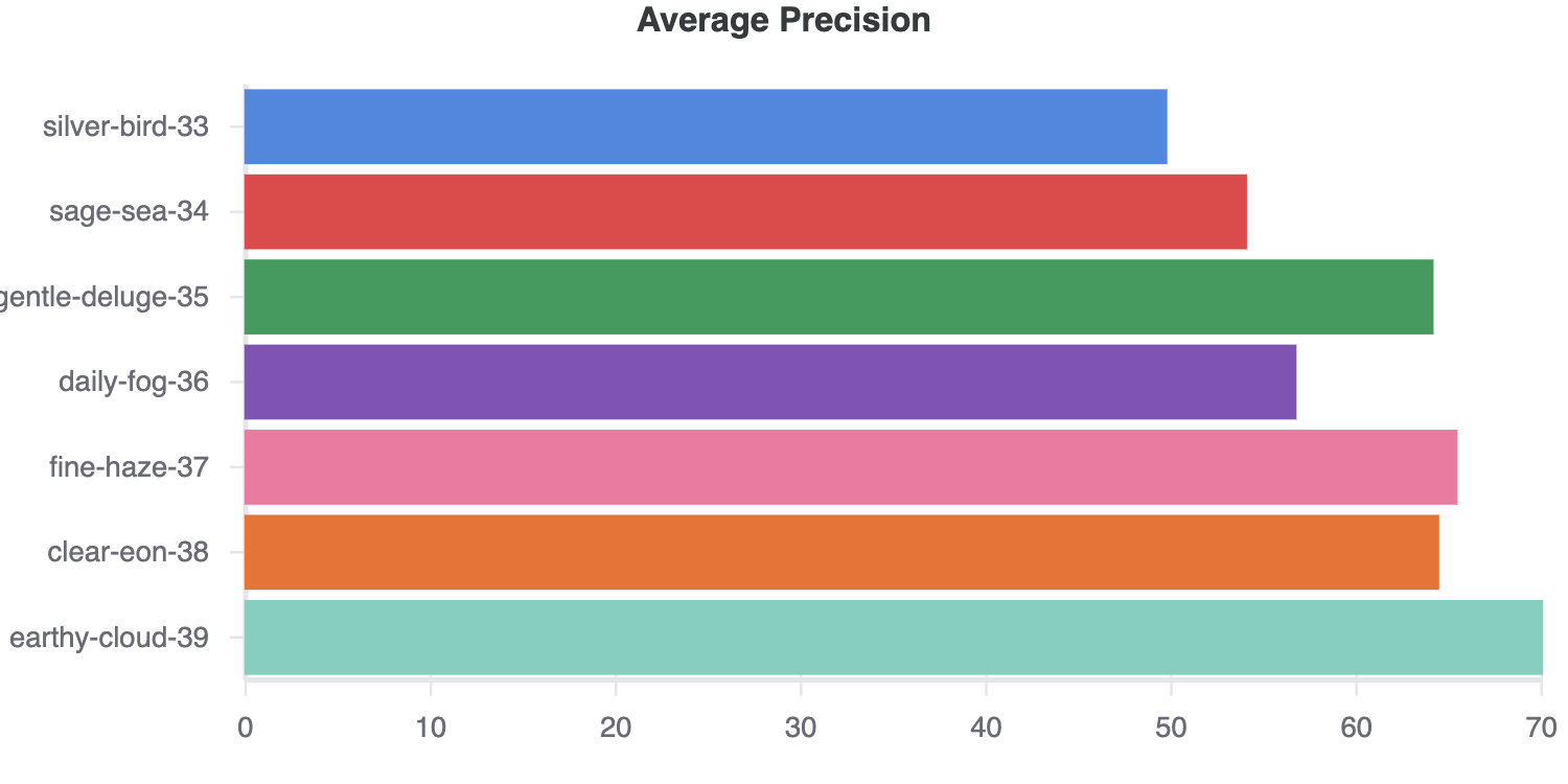
I ran the experiment. And thanks to Weights & Biases, the outcome was beautiful.

Why?

Because the models showed they were learning something (the average precision, a metric for evaluating object detection models was improving) and there weren’t any outlandish differences between each of the models (meaning the experiment controls worked).

Then what?

To narrow things down and see which model I should use to build a big dog model (a model with all the data and trained for longer), I hypothesised another experiment.

I’d take the top two models from my first experiment, retinanet_R_50_FPN_1x (fine-haze-37) and retinanet_R_101_FPN_3x (earthly-cloud-39), train them both a reasonable amount of time (about 1000 iterations) on a larger dataset (10% of all the data) and then compare the results.

# My second modelling experiment in pseudocode
for model in top_2_models: 
    with random_seed x
    do 1000 iterations 
    on 10% of the total data 
    save results to Weights & Biases

Then whichever model came out on top would become the big dog model.

It must be known, since I was on my own imposed deadline (42-days for the total project), experimenting quickly was paramount.

In the Airbnb article, they mentioned they trained their models for 5-days and 3-days at a time. Since I’d allocated ~10-days to modelling total, I really only had 1 shot at training a big dog model.

By this stage, I’d downloaded the entire training, validation and test datasets from Open Images. And to run the second major experiment, this time I’d decided to compare the two best performing models on a portion of the whole dataset (all 30 target classes rather than only 3 classes).

Dataset status:

• 34,835 training images
• 860 validation images
• 2,493 test images

When running modelling experiments on small portions of your data it’s important the small portions are of the same distribution as the full data.

In other words, if you’re going to run a modelling experiment on 10% of the data, make sure that 10% of the data has the same class distribution as the full dataset. In the case of the Airbnb dataset, if the full dataset has plenty of images of staircases but not many images of wine racks, the smaller version should echo this relationship.

I made the 10% training data split by randomly selecting examples from the full dataset and ensuring the distribution of classes looked similar.

# Get 10% of samples from train dataset
small_dataset = full_dataset.sample(frac=0.1)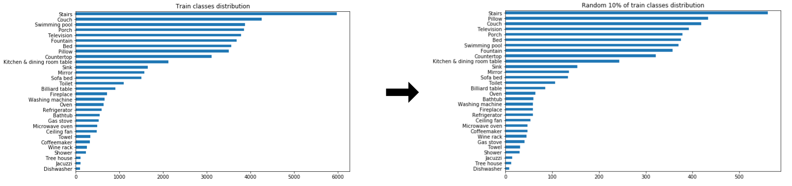

I also ended up merging the validation and test sets from Open Images into one dataset val_test. The reason for this being Airbnb mentioned they used a 10% test data split for evaluation (75k total images, 67.5k training images, 7.5k test images).

Dataset status:

• 34,835 training images
• 3,353 test images (original validation and test set images merged)

With the smaller representative datasets ready, I kicked off the second major experiment, ensuring to track everything in Weights & Biases.

As it turns out, both models performed well, meaning the metrics that should go up (average precision) were going up and the metrics which should go down (loss) were going down. Despite the 10x increase in the number of classes, my models were learning (a good thing).

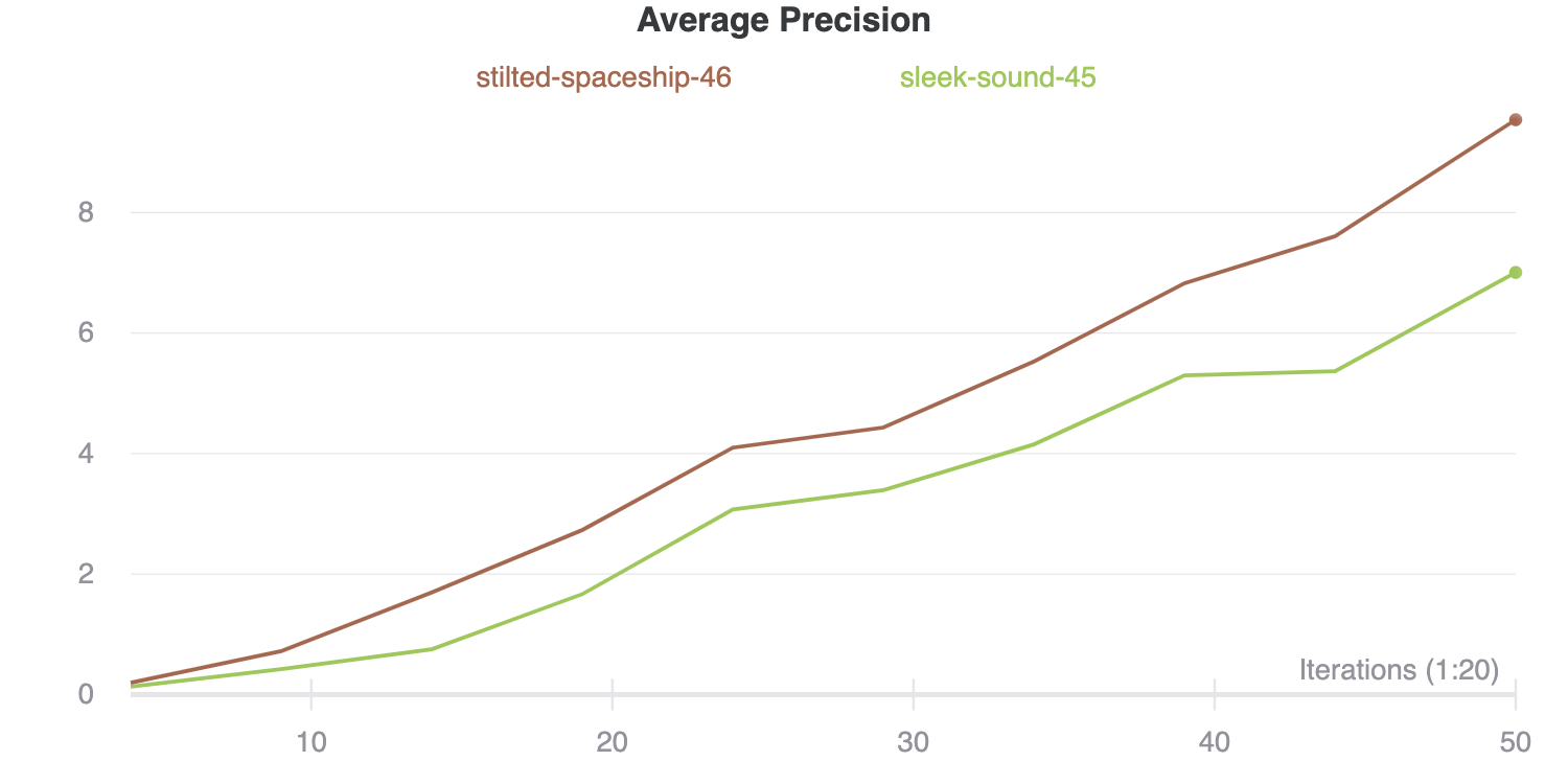
Based on the results of my second major experiment, I ended up deciding retinanet_R_101_FPN_3x (stilted-spaceship-46) would be upgraded to big dog model status.

Training a big dog model (a model trained on all the data)

• Ingredients: 38,000+ Open Images (all of Airbnb’s target classes)
• Time: 3 days of human time, 18-hours compute time
• Cost: $150-175 ($1.60/hour P100 GPU + multiple fails + under-utilised instance)
• Utensils: Weights & Biases, Detectron2 retinanet_R_101_FPN_3x

Detectron2’s pre-trained models were trained on Big Basin (a big dog computer with 8 GPUs). I didn’t have 8 GPUs (graphical processing unit, a computer chip capable of fast computations), so far, everything I’d done had been on Google Colab (1 GPU) or my local computer (no GPUs).

Based on my previous experiments, training with 10% of the data for 1000 iterations, I knew a full training run on the whole dataset using 1 GPU for 100,000+ iterations (taken from Airbnb’s article and Detectron2 model configuration files) would take about 15 to 20-hours.

With this back of the envelope time line calculation, I figured I’d only really have one shot at training a big dog model.

Originally, I’d intended to do some hyperparameter tuning (adjusting models settings for better results) but due to the constraints didn’t spend as much time here as I would’ve liked.

So I decided to focus on only a couple:

• Learning rate (how much the model tries to improve its knowledge at any one time).
• Mini-batch size (how many images the model looks at one time).

In my experience, aside from the structure of the model itself (layers, etc, already decided by Detectron2 anyway), these two settings are the most influential in performance.

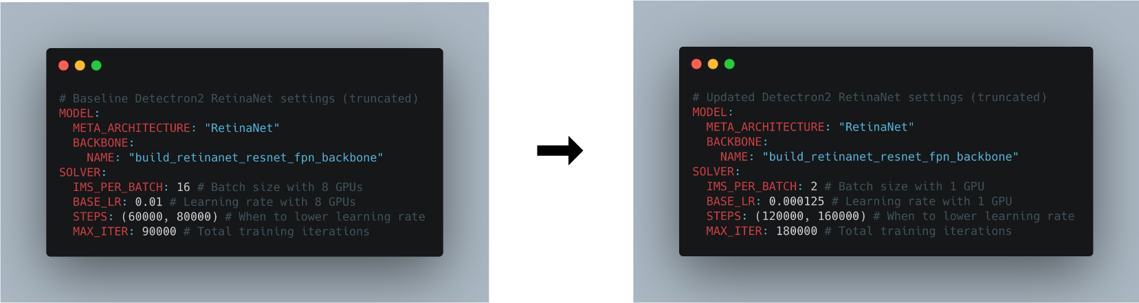
I stumbled across the linear learning rate scaling rule, read up a little more about it and decided to apply it to the retinanet_R_101_FPN_3x model's base settings.

The linear learning rate scaling rule says your batch size and learning rate should increase and decrease with the number of GPUs you’re using.

For example, since I was using 1 GPU versus Detectron2’s original 8 GPUs, if adhering to the rule, I should divide the original learning rate and mini-batch size by 8.

# Linear learning rate scaling rule
new_learning_rate = old_learning_rate/(new_num_gpus * old_num_gpus)

I adjusted the settings accordingly, and since I was using transfer learning (not training from scratch), I divided the new learning rate by a further multitude of 10.

Why?

I read in the Airbnb article when they tried transfer learning, they divided the learning by 10 as a precaution to not let the original model patterns be lost too quickly whilst the new model learned.

This intuitively made sense to me, however, I’m sure there is either a better way to do it or a better explanation. If you know, please let me know.

Well, 18.5-hours, 34,834 training images and 180,000 training steps on a P100 GPU later, my model finished with a mAP (mean average precision) score of 43.297% on the held-out test set.

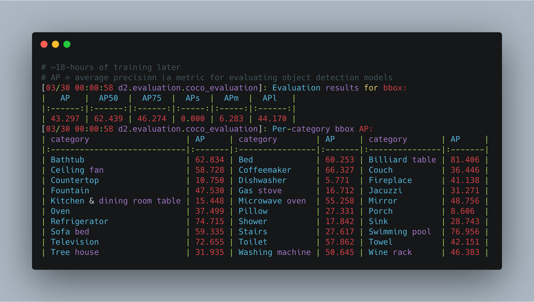
Lower than Airbnb’s result of 68% mAP using Google’s AutoML but higher than their results of using transfer learning.

In should be noted though, these metrics (mine and Airbnb’s) aren’t really comparable since we used different datasets, me having only access to public data, Airbnb having public and internal image data.

But metrics schmetrics, right?

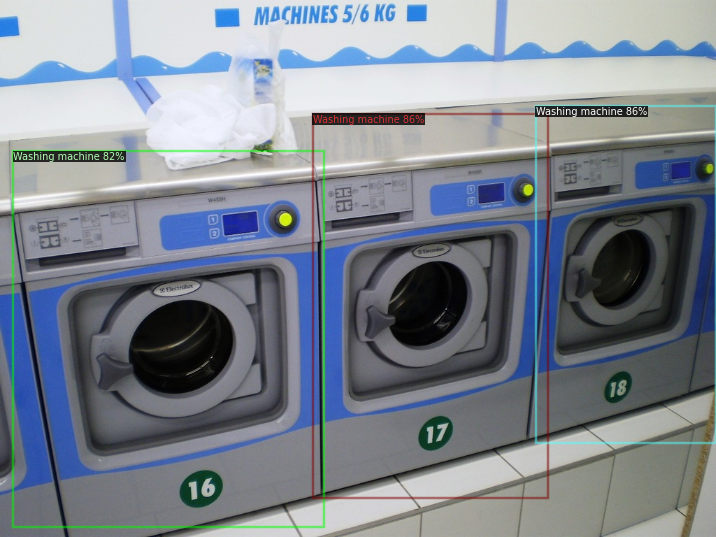
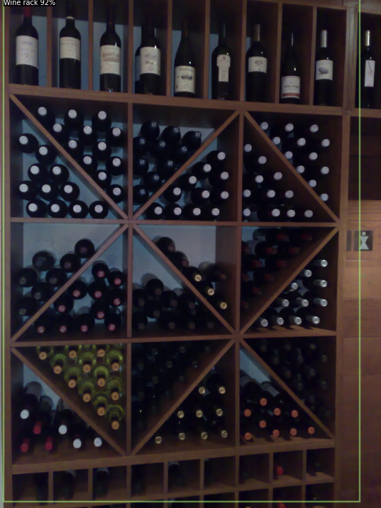
The real test of a computer vision model is on actual images. Let’s look at a few from the test set (remember, the model has never seen these before).

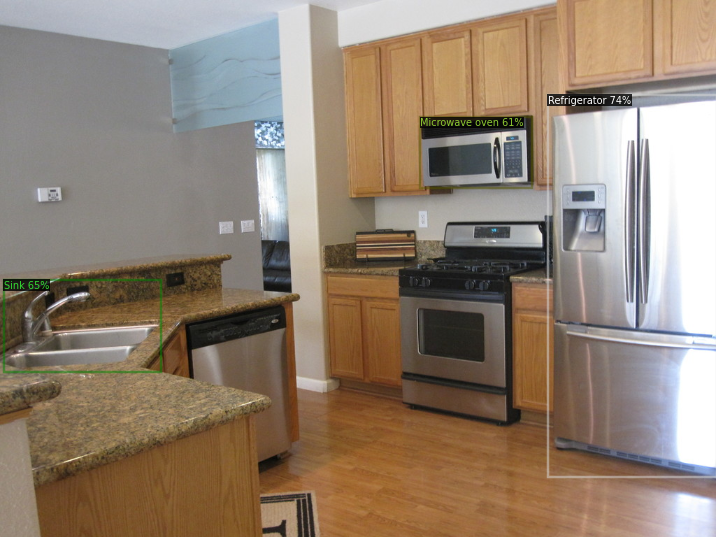
And how about on some custom images, courtesy of my bedroom and kitchen?

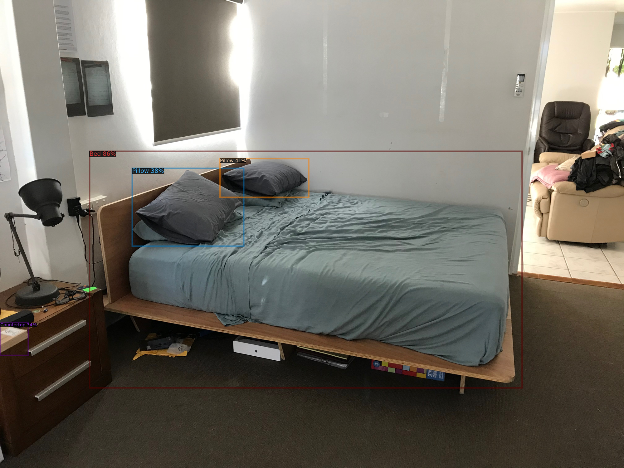
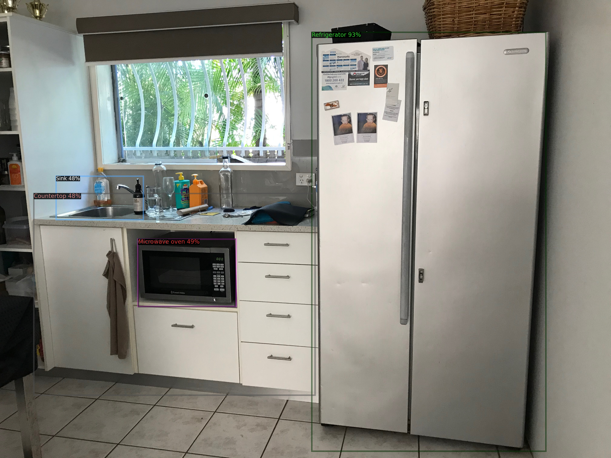
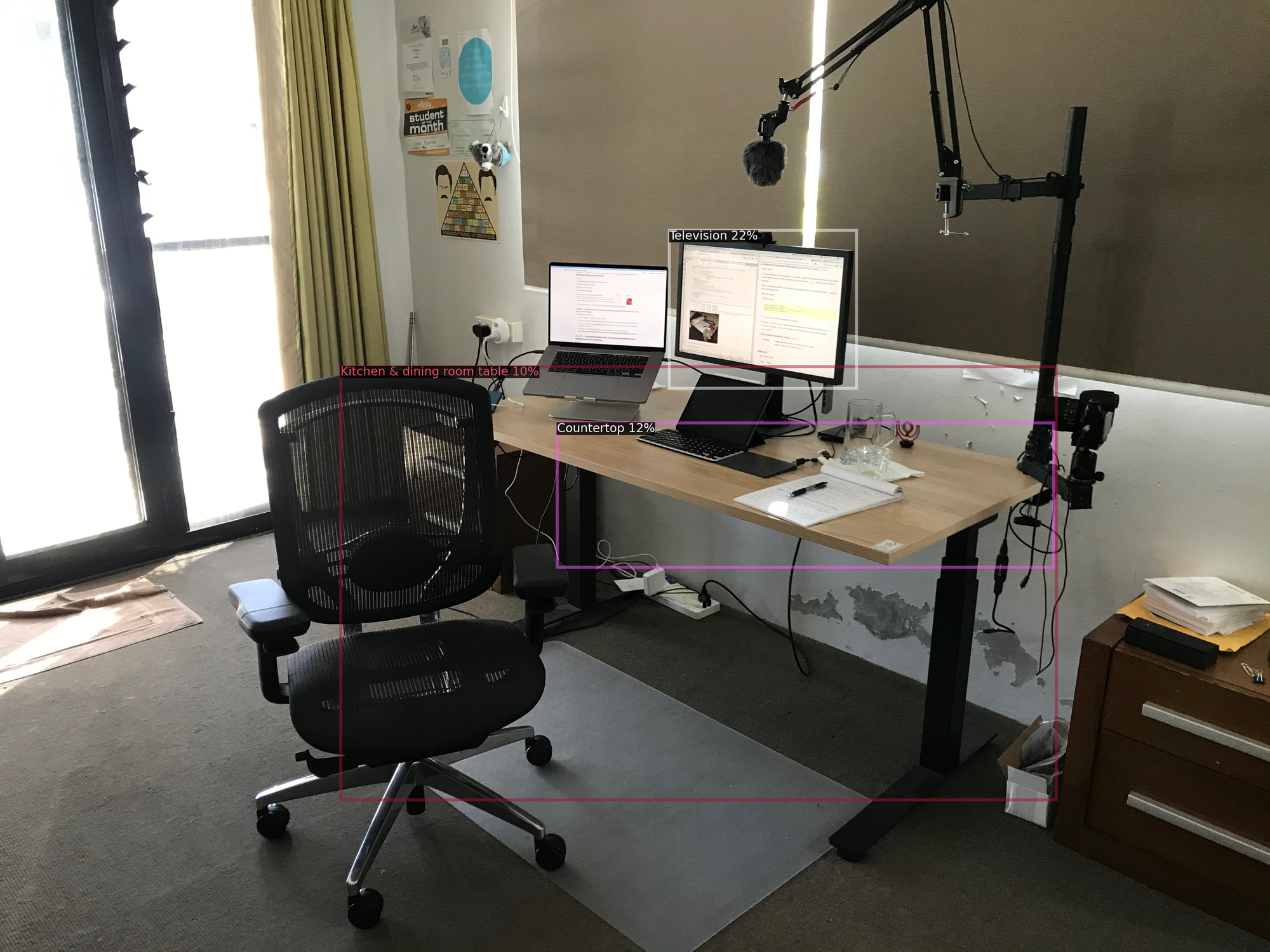
Seeing a machine learning model work on stock data: Hey that’s pretty cool…

Seeing a machine learning model work on your own data: OMG WHAT IS THIS MAGIC???

With modelling completed (as much as the time would allow for), it was time to get it live.

App building and deployment: A custom model in Jupyter is cool but being live on the web is cooler

• Ingredients: Fully trained custom machine learning model
• Time: 4 days
• Cost: $14 hosting per day (I know, I need to fix this)
• Utensils: Streamlit, Docker, Google Container Registry, Google Compute Engine

Machine learning model deployment still seems like a bit of dark art.

First of all, coding in Jupyter Notebooks is different to writing Python scripts. Then you’ve got the different packages you need, from data science libraries to web frameworks. Then you’ve got to build some kind of interface around your model a user can interact with. Once you’ve done that, where do you host it?

All challenges worth taking on for any budding machine learning engineer.

After all, if a model only exists in a Jupyter Notebook, does it exist at all?

If you’re a Jupyter Notebook warrior like me, the good news is, Streamlit and Docker are here to help you.

Streamlit helps you build a user interface for your machine learning and data projects. Even better, it’s all in Python too. If you’ve never tried it, go spend half a day going through all the tutorials and you’ll be set.

Now Docker. Docker helps you wrap all of your files (Streamlit app, machine learning model and dependencies) up into a nice little package (called a Docker Image). Once you’ve got this package you can upload it to a cloud server (e.g. Google Cloud) and everything goes right, it should run exactly how it does on your local system.

So you’ve got a trained model making inference in a Jupyter Notebook? Your workflow to deploy it could go something like this (what I did):

1. Create a folder called something like app. This is where your Streamlit app (a Python script), model artefacts and all other required files will live.
2. Create a completely new Python environment in the new folder. You’ll want to install the barebones dependencies for your app to run in this. In my case, I needed Streamlit and Detectron2’s dependencies.
3. Build a Streamlit app around your model (a Python script).
4. Get the Streamlit app working locally. This means you can interact and see the app working on your computer.
5. Create a Docker Image of your environment and app folder.
6. Upload your Docker Image to Docker Hub or a Docker hosting service such as Google Container Repository.
7. Use a cloud provider such as Heroku, Google Cloud or AWS to host and run your Docker Image.

If everything goes right, you should be given a URL to your hosted app.

Since I used Google’s App Engine, mine came out looking like this: airbnb-amenity-detection.appspot.com

We covered app building and deployment very quickly. But if you’re interested in learning more, I’d check out the following resources (in order).

• How Docker Can Help You Become A More Effective Data Scientist by Hamel Husain
• Streamlit deployment references (AWS, Heroku, Azure)
• How to deploy Streamlit apps to Google Cloud Platform by JarvisTech

Criteria and evaluation: Comparing my model to Airbnb’s

I started this project with a series of criteria I wanted to fulfil.

Let’s review them.

• ✅ Have the app accessible to someone on their mobile device. This works but is janky. Despite the jankiness, it gets a tick.
• 🚫 Beat or at least equal Airbnb’s MVP of 50% mAP. None of my models reached or passed this threshold. So this is a fail.
• ✅ Fix the pain point of not being able to download the AutoML model Airbnb used. My fully trained Detectron2 model is available for download and usable by anyone. Tick.
• 🚫 Have some sort of way to find the images/classes a model is most uncertain about. You can kind of do this by looking at the evaluation metrics print outs but I was thinking more of a visualizer function to move towards an active learning approach for classes/images which perform poorly. Fail.
• 💰How cost-effective is running the model? For this one, let’s get out the notepad.

After watching a video on machine learning at Airbnb, someone mentioned they’ve got upwards of 500,000,000 images on the site (yes, 500+ million). For our calculations, let’s pretend we’d like to run our model across all of them.

With the retinanet_R_101_FPN_3x model I trained and the GPU I used (a Nvidia P100) it took about 0.2s to make a prediction on each image.

• GPU cost: $1.46/hour (GCP, us-central1), $0.0004/second
• Inference time: 0.2s/image, 5 images/second
• Total number of images: 500,000,000
• Total inference time: 100,000,000 seconds (500,000,000/5)
• Inference cost per image: $0.000081
• Total inference cost: $40,555.55
• Total inference time (1 GPU): 27,778 hours (1160 days).

Of course, more calculations would be required to see how much value the model adds could be done. But seeing these gives you an idea of how much a proof of concept would be across all of Airbnb’s images.

It's quite clear, in the current state, using the model across all of Airbnb's 500,000,000+ images is probably not viable.

However, these numbers were also calculated using 1 rented GPU on Google Cloud. If a local machine had multiple GPUs, the costs (and time) could be decreased dramatically.

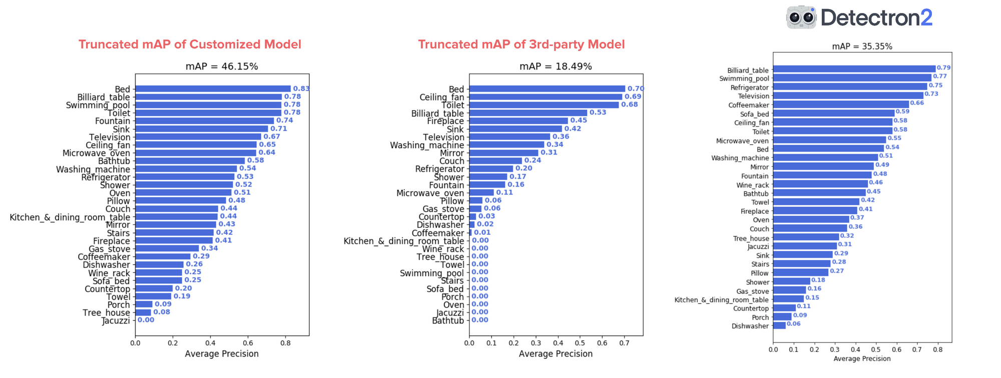
The final comparison worth looking at is the final one Airbnb used in their article. They started their project as a way to build their own custom computer vision model which would save them from using 3rd-party amenity detection services.

They noticed the 3rd-party amenity detection service only showed results for predictions with a confidence score over 0.5 (the higher the score, the more confident a model is behind what it’s predicted). So to make a fair comparison, they altered their Google AutoML model to do the same.

Doing this, the results from Airbnb’s Google AutoML model went from 68% mAP to 46%. Seeing this, I did the same with my model and found the results went from 43.2% to 35.3%.

Extensions, potential improvements and takeaways

Of course, this project isn’t perfect. But I wasn’t expecting it to be. I’m a cook, not a chemist.

I would’ve liked to have done a few more things before the end of the 42-days, such as:

• Hyperparameter tuning. Despite my model performing pretty well, I didn’t do as much hyperparameter tuning as I’d liked. If I was going to, I’d probably turn to Weights & Biases Sweeps (a tool for trying, tuning and tracking hyperparameters). With tuned hyperparameters, who knows, maybe my model could’ve turned out 1–5% better.
• Reduced inference time. As seen when calculating the business use-case costs of the model, for it to be run at scale (on all of Airbnb's images), inference time would either need to be dramatically decreased or more processing power (more GPUs) used. While working on this project, EfficientDet, an efficient object detection algorithm was released. So that's probably what I'd try next.
• Labels created on download. Preprocessing Open Images data to work with Detectron2 takes a few steps which could probably be automated when downloading images in the first place.
• A less janky app (my fault, not Streamlit’s). I’m still getting used to deploying the code I’ve written in a Jupyter Notebook. In the future, I’d also like my own server I could push Docker containers to and share with others.
• A retraining pipeline. How could I easily retrain a model if more images or classes were added? Right now, this would take almost rerunning the entire project.
• Inspection functions. If I wanted to inspect the data and look at things such as all the images of Kitchen & dining room tables or all of the images with predictions below a certain confidence threshold, I can’t. These kinds of visualizer functions would be paramount for further data exploration (and perhaps should’ve been built at the start).
• What images have people in them? Because I used Open Images, many images have people in them. A cascade of models could be used to filter out unwanted styles of images and only focus on the ones related to Airbnb’s use case.

With all this being said, the project achieved its main goal: learn by doing.

I learned a bunch about a handful of tools I’d never used before and even more important, how I might go about structuring future projects.

The main takeaway(s) being, experiment, experiment, experiment.

See how it was done

Despite the length of this article, it’s a short overview of the actual steps I took during the project.

If you’d like to see them all unfold, you can read my project notes (in daily journal style) in Notion.

Or watch the YouTube series I created to go along with it.